Dave Bulman, School of Geography and Environmental Science, Monash University and Cooperative Research Centre for Weed Management Systems, Clayton, Victoria 3168, Australia.
Current address: Army Engineering Agency, Support Command Australia (Army), Private Bag 12, PO Ascot Vale, Victoria 3032, Australia. E-mail: dave.bulman@aea.sptcomd.defence.gov.au
The play on words expressed in the title underlies a more significant question regarding the prospects for using remote sensing technology to map the extent of environmental weeds that seriously impact on agriculture: How realistic is the expectation that remote sensing can become routinely applied to weed mapping? This paper presents an overview of remote sensing and how it works, examines how it has been used for land and resource evaluation and monitoring, and describes briefly some of the inherent difficulties associated with its application to weed mapping using, as an example, research on mapping Paterson’s curse, a weed of perennial pastures. An explanation is given about some of the key factors relating to the spectral characteristics of the weed, and its behaviour in response to natural and human factors and shows that infested areas can be mapped but that determining weed distribution and density are not always possible using currently available remotely sensed data. In particular, it demonstrates that the use of high resolution data solves some of the difficulties encountered when lower resolution data are employed for weed mapping. In conclusion, it points to answering the above question with the proposition that: Much depends upon the characteristics, behaviour and environments of the weeds; and future developments in remote sensing technology.
The applications for remote sensing continue to increase and will most probably go on doing so with progressive improvements in the technology. A large range of applications already exist for remote sensing in areas as diverse as land cover mapping, geology, marine and terrestrial resource evaluation. In 1995 ABARE listed some 120 separate applications for remote sensing (Watson et al. 1995), while a Bureau of Rural Resources survey in 1990 list some 136 separate remote sensing projects in agriculture alone (Kelly et al. 1990). These statistics are testament to the economies of scale that can be achieved in thematic mapping where areal coverage using satellite imagery can be extensive and, on a per unit area basis, relatively inexpensive. But technological limitations still constrain its employment for routine or ‘operational’ usage in many cases. These limitations are primarily imposed by the lower spectral and spatial resolution of satellite data on the one hand, and the greater expense of conducting air-borne surveys to obtain higher resolution air-borne data on the other. Although much can, and has been achieved in remote sensing, the limits imposed by current technology still prevent its routine application for some areas of land and resource management. This is particularly the case for weed mapping, where frequently the patterns of their distribution stretch the limits of spatial and spectral resolution available from current satellite data and is generally too expensive for the more appropriate air-borne mapping. It is of no great surprise then, that of the 136 agricultural applications for remote sensing in Kelly’s report, only three were related to weed mapping. Improvements in the spectral and spatial resolution of remote sensing data and the increasing number and coverage of satellites and air-borne instruments, will provide greater opportunities for detecting, mapping and managing the environment and earth resources including that of some of our most widespread and worst weed problems.
In order to better understand the limitations of current remote sensing technology referred to above, some basic ideas about how remote sensing works is provided. This paper gives a brief overview of the nature of remote sensing, examples of how it is being used and some of the limitations encountered when applied to weed mapping, drawing on my research into mapping Paterson’s curse in north-east Victoria.
By one definition, remote sensing is a means of collecting information about objects or phenomena by indirect measurement – that is by no direct interaction with the object of study. Perhaps the earliest form of remote sensing was conventional photography, and was utilized soon after its invention for obtaining information about the Earth’s surface. While photography is still used extensively for mapping and detailed surveying, remote sensing has come to mean more specifically the recording of reflected electromagnetic energy from objects on the Earth’s surface electronically rather than on film providing scope for a broader range of applications. Other forms of remote sensing make use of video (in the visible and infra-red bands) and radar (in the microwave bands) but these won’t be considered here.
Electromagnetic spectrum
Objects illuminated by the sun will absorb electromagnetic radiation (light) of certain wavelengths and reflect others. Light reflected in the visible light bands give objects their colour. However, many objects also reflect light in other parts of the spectrum and of particular interest to earth scientists are the infra-red wavelengths. The amount of reflected light at various wavelengths provides a means of distinguishing different objects. Figure 1 illustrates the percentage of light that is reflected from three general land surface types at the wavelengths covered by the majority of remote sensing instruments. Variations in these curves provide the means to determine differences between different land cover types, such as vegetation, soil and water, on the basis of their characteristic reflectances.
Figure 1. Electromagnetic spectrum showing reflectance for major land cover types and the bands used for Landsat TM (Source: Richards and Jia 1999).
On-board detection of reflected light
The intensity of reflected energy from different surfaces is recorded by an on-board instrument, called a spectrometer, at several wavelengths depending on the particular instrument. In the case of satellite instruments, for example Landsat, seven bands of data are collected – three in the visible light and four in the infra-red bands. Six of these bands are indicated by the numbers 1–5 and 7 in Figure 1. Band six, not shown in the figure, collects data from the thermal part of the infra-red spectrum at much longer wavelengths and is used for more specialized analysis.
Recording in digital form
The radiation collectors or sensors record the levels of reflected energy and convert the data to digital form for transmission to ground receiving stations where the data is then processed and archived. It then becomes available for purchase by potential users.
Satellites and air-borne instruments
Spectrometers, can be carried on board satellites as well as on specially fitted aircraft, such as those that might alternatively carry aerial photographic equipment. Many air-borne instruments can be ‘tuned’ to collect data from a larger number of user-defined bands than is available from satellite instruments. This improves the ability to better discriminate the features of interest. The Compact Air-borne Spectral Imager (CASI) is one such instrument that has the ability to collect data from up to 228 bands concurrently. Hand-held spectrometers can be used to collect detailed spectral data in the field for calibration or comparison.
As the satellite or aircraft passes over the land surface, an array of sensors in the spectrometer sweep across the landscape collecting data in a swathe which can be up to 185 km wide in the case of Landsat and variable from about 2–10 km for air-borne instruments depending on aircraft flying height. Data is collected simultaneously from the array of sensors each of which records data from a unit of the land surface known as the instantaneous field of view (IFOV). For Landsat the IFOV is about 32 m and for CASI is, again, determined by flying height to be between 1 and 10 m. It is the dimensions of the IFOV that determines the important characteristic of ‘spatial resolution’ of remote sensing data, while the number and spectral width of the bands of data collected determine the ‘spectral resolution’.
Remote sensing data visualization and analysis
Data from remote sensing instruments is utilized in basically two ways by analysts (Richards and Jia 1999). The digital data can be displayed on a computer monitor in the form of an image re-constructed from the individual data components collected from the array of sensors. When they are arranged and displayed in the correct spatial configuration as they occur on the ground they become the individual picture elements or ‘pixels’ that make up the total image. Since a colour computer monitor is only capable of displaying three channels at one time, a choice is made as to which bands will be displayed in which channel.
Display of images and data visualization
By displaying the three visible light bands in the red, green and blue channels on a computer display, a more or less ‘natural’ colour image is formed that closely approximates the impression that one has from the air (Figure 2a). But there are many possible combinations of displaying three of the six usual Landsat bands used for most analysis. Wide use is made of displaying one of the infra-red bands in either the red channel or in the green channel. In the former case a ‘false’ colour image is generated where the strong infra-red reflectance from vegetation (see Figure 1) is used to enhance the visual representation of vegetation that is more strongly red the more vigorous the growth (Figure 2b). In the latter band configuration vegetation takes on a more natural green colour but with enhanced separation from other land cover types.
|
|
|
Figure 2. (a) Landsat TM image using a ‘natural’ colour composite of bands 1, 2 and 3; (b) False colour composite incorporating an infra-red band in the red channel.
The various combinations possible provide the analyst with a means of examining and interpreting the imagery for particular features and to study the patterns of colours to gain an appreciation of the scene content in terms of land cover types and their variation. Many subtle variations in colour can often be identified by experienced analysts as belonging to a particular class of land cover or as being at a particular stage of plant growth or condition.
Numerical image data analysis
While visual interpretation of image data is a valuable exercise in determining the existence of particular phenomena of interest, often more rigorous methodologies are required to either enhance the display or to extract more detailed information about the land cover types of interest. There are many ways to enhance the display of imagery. Band ratio methods are often used, for example, to express important relationships between the bands that are known to show certain phenomena. Green vegetation indices are often used to show plant vigour as a measure of water availability, the onset of drought or the risk of fire. Figure 3, for example, shows one of a monthly series of mappings of a vegetation index to monitor the state of drying out or greening up of vegetation on a continental scale. Many such band relationships and transforms are used for land cover mapping, environmental research and monitoring, soil mapping and in geology for mineral identification. These are all based on known relationships between the numerical values in each band.
Figure 3. Normalized Difference Vegetation Index (NDVI) map showing the state of vegetation ‘greenness’ monitored on a regular basis by Environment Australia (Source: Bureau of Meteorology (copyright) http://www.gov.au/sat/archive_new/ndvi/).
These numerical relations and the image statistics can be extended to express features and phenomena that cannot be readily visualized at all in the raw data, when such patterns can only be revealed after mathematical analysis. In Figure 4 the visual results of an analysis for soil attributes such as pH, salinity and texture (where each colour represents a level of the particular attribute, salinity in this example) are displayed.
Perhaps the most significant analytical technique applied to remote sensing imagery is that of pixel classification. The object of such analyses is to group individual pixels in an image into a number of classes based on spectral similarity – that is, based on the similarity of values recorded in each band – such that each class can be recognized as a particular type of land cover feature. Figure 5 shows the results of an image that has been classified into categories according to their agricultural potential, overlaid with cadastral information about property boundaries.
|
|
|
| Figure 4. Satellite imagery analysed to show soil salinity patterns. (Source: Goulay 1996a). | Figure 5. Image classified to show soil properties related to land capability (Source: Goulay 1996b). |
The 121 applications for remote sensing listed by Watson et al. (1990) are divided into some 16 categories of which the following include the main areas for which remote sensing has been employed:
Since it would be impractical to illustrate examples for many of these, the following images provide some idea of the diversity of applied remote sensing to land and environmental studies:
Environmental monitoring Figures 3 and 4 show some typical applications where temporal sequences of regular images can be used to monitor changes in the environment. Such series of images can be used to examine the effects of activities such as forest clearing or to monitor the effectiveness of tree planting programs to ameliorate erosion or salinity.
Land resources Figure 5, referred to earlier, provides a means to access the productive potential of land and can sometimes highlight areas where potential problems such as erosion, water-logging and salinity might occur.
Geology and geophysics Figure 6 illustrates the application of image enhancement methods to improve the visualization of geological features and their mineral content.
|
|
|
| Figure 6. Satellite image analysed to show geological mineralization (Source: Coker and Sanders 1998). | Figure 7. Shallow water mapping showing water depth and flow patterns (Source: Bierwirth 1996). |
Marine studies Figure 7 is an application of remote sensing to shallow water mapping in a coastal zone for mapping water depth and flow patterns. Weather and climate Figures 8 shows the familiar satellite imagery used to supplement weather prognostic charts. The application of remote sensing to weed mapping Weed characteristics and data parameters In order to successfully apply remote sensing technology to weed mapping, there must be some characteristic of the weed of interest that permits its spectral discrimination from other species with which it is associated. Such features as distinctive leaf shape, floral characteristics or phenological attributes need to be defined that allow the target weed to be distinguished from its associates at certain stages during its life cycle or under certain environmental conditions. In conjunction with this, consideration must be given to the spatial arrangements of weed patches. The spectral signal from a plant that grows in patches smaller than the spatial resolution of the remote sensing imagery may be significantly ‘diluted’ by the signal from the major land cover within a given pixel, thus reducing its ability to be detected. These ideas are illustrated in Figure 9a where, for example, patches of flowers are set in an otherwise uniform background of green. At the scale of the Landsat resolution of 30 m, the spectra from the flowers would be overshadowed by the background signal while for a higher spatial resolution such as might be obtained from an air-borne scanner at 2 m resolution (Figure 9b) there would be at least some pixels with a much higher density of floral elements and therefore more likely to be detectable.
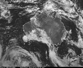
Figure 8. Satellite images used for weather forecasting and prognosis (Source: Bureau of Meteorology (copyright). http://www.bom.gov. au/weather/national/satellite/).
|
|
|
| Figure 9. (a) Relationship of target species patch relationship to IFOV for a spatial resolution of 30 m, and (b) The improved chance of obtaining target species signals from a higher spatial resolution of 2 m. Inset show detail of selected pixel contents with higher density of target. | |
Spectral resolution is a function of the number of bands available, their location in a part of the spectrum where the greatest discrimination of the characteristic feature is possible, and bandwidth of the bands used. As can be seen from Figure 10, which shows the spectra both for flowers of Paterson’s curse (Echium plantagineum ) and the vegetative parts of the plant, that the bands of Landsat satellite instruments are much broader than those of the CASI air-borne instrument. Moreover, the critical band, the green band, overlaps the region of greatest spectral difference where there is lowering of the green reflectance for the flowers compared to the vegetative components of Paterson’s curse . The narrower bands of CASI allow a more targeted positioning of where spectral information can be collected from so increasing the possibility of discriminating Paterson’s curse from its background.
Figure 10. Spectral characteristics of Paterson’s curse flowers versus the vegetative parts of the plants with the positioning of bands from Landsat TM and CASI instruments. (Courtesy CSIRO Land and Water).
Environmental considerations
In addition to the technical and biological considerations, environmental factors also have an important influence on the ability to successfully detect and map a weed of interest. This is particularly the case if one is interested in using remote sensing for a long term study of weed distribution, or periodic changes in patterns of infestation. Among the many possible influences on year-to-year plant behaviour are seasonal climate variations, landuse changes, management practices and weed control practices. These factors can influence phenological relationships and plant responses, while the timing of grazing with respect to timing of data collection and the implementation of weed control measures can result in variations in the ability to detect the target species in an image.
Outline of Paterson’s curse work It is perhaps fortunate that Paterson’s curse produces flowers that have a distinctive colour which few other pasture species possess. In 1988, use was made of this to demonstrate the potential for use remote sensing imagery to detect and map this weed (Ullah et al 1989). The current project aimed to extend this potential into a practical method to routinely map and monitor Paterson’s curse distributions. It soon became apparent, however, that some of the factors outlined above would hinder progress toward this end. Not least of the factors were those related to the scale of weed patchiness and the matters of data spectral and spatial resolution.
Some results
While re-examination of the 1988 image still produced a quite clear pattern of Paterson’s curse distribution (Figure 11), no such pattern was as evident in the years from 1996 through to 1998 (Figure 12) for images acquired for the same time of year. In 1998 I was able to obtain some CASI data in a joint mission conducted by CSIRO Land and Water (Byrne personal communication) at 1 m spatial resolution and with bands targeted to discriminate more precisely the spectral properties of Paterson’s curse (Figure 10). Figure 13 shows the results of classification for Paterson’s curse (shown as the magenta overlay) of the Landsat image for 1998 (Figure 12 - a section of which is shown in the left panel) and the results from analysis of the CASI data (Figure 13 - right panel). The ‘blocky’ results for the Landsat image indicate that the patchiness of Paterson’s curse does not match the image resolution and perhaps overestimates its extent producing a confused pattern, while more realistic patterns, can be achieved by the analysis of data obtained at higher spatial resolutions, aided by a better ability to spectrally discriminate the floral components from the background.
|
|
|
| Figure 11. Landsat TM image of the Lake Hume study area for 1988 showing Paterson’s curse infestations in the magenta colour (arrows). | Figure 12. As for Figure 11 in 1998, taken at the same time of year, with no clear indication of Paterson’s curse in spite of its presence on the ground. |
Figure 13. A comparison between classified Landsat data for one survey site (scaled up from Figure 12) in 1998 (left) and that of the CASI data (right) for the same time showing the improvement in Paterson’s curse detection from the higher resolution data.
Acknowledgments
The research on mapping Paterson’s curse was conducted while in receipt of a Monash Graduate Scholarship with supplementary support from the Cooperative Research Centre for Weed Management Systems. The author acknowledges the contribution of CSIRO Land and Water to the collection and preparation of CASI data. Permission by the respective authors to use images published in GISUser is gratefully acknowledged as is helpful comments by E. Ullah and J. Peterson on an earlier draft of this paper.
References
Bierwirth, P. (1996). Imaging the sea bottom from space. GISUser 16, 25-7.
Coker, J. and Sander, A. (1998). The use of remotely sensed data in geological mapping. GISUser 25, 36-7.
Goulay, R. (1996a) Mapping soil properties. GISUser 15, 30-2. Goulay, R. (1996b). In pursuit of precision farmers. GISUser 17, 42-3.
Kelly, G., Hamblin, A. and Johnston, R.M. (1990). Remote sensing for agricultural production and resource management in Australia. Bureau of Rural Resources Bulletin No. 8, 70 pp. AGPS,
Canberra. Richards, J.A. and Jia, X. (1999). ‘Remote Sensing Digital Image Analysis’, Third edition, 363 pp. (Springer-Verlag).
Ullah, E., Shepherd, R.C.H., Baxter, J.T. and Peterson, J.A. (1989). Mapping flowering Paterson’s curse (Echium plantagineum) around Lake Hume, north eastern Victoria, using Landsat TM data. Plant Protection Quarterly 4, 155-7.
Watson, W., Anandajayasekeram, P., Miller, E., Allen, R., Curtotti, R., and Johnston, R. (1995). Remote sensing: use in agriculture and resource management: A conceptual framework for economic analysis. ABARE and Bureau of Resource Sciences Research Report 95/5, Canberra, 80 pp.
Editor’s note: The correct citation for this paper is Bulman, D. (2000). Is the application of remote sensing to weed mapping just ‘S-pie in the sky’? Plant Protection Quarterly 15, 127-131